A Laser Wakefield Accelerator

Last updated on 2026-09-23 | Edit this page

Overview

Questions

🏄 How can electrons catch a ride on a laser-driven plasma wave?
🧩 How do particles, a grid, and a moving window bring this system into the computer?
🔍 What can we discover in the density, electric-field, and energy plots?

Objectives

🔦 Identify the laser, plasma target, and wake in a reduced 3D simulation.
📏 Connect spatial and temporal resolution to the scales of the laser and plasma.
🚀 Run WarpX and visualize saved field and particle diagnostics.
🕵️ Distinguish evidence of a wake from evidence of a usable accelerated bunch.

Surfing a plasma wave

Imagine electrons surfing a wave, with a laser providing the push that creates it. 🏄 The wave here is a pattern of charge and electric field in a plasma, and riding the right part of it can give electrons energy.

A plasma contains free electrons and ions. An intense laser pulse pushes electrons out of its path. The heavier ions respond much more slowly, so the separation of positive and negative charge produces an electric field. The electrons move back toward the ions and can oscillate, leaving a wake behind the pulse. Electrons traveling in the appropriate part of that wake can gain energy from its electric field. This is laser-wakefield acceleration.

WarpX can model how a laser and plasma evolve together and how electrons respond to the resulting fields. Read Introduction to WarpX for the particle-in-cell (PIC) method. Here you will launch a laser into a small plasma target, watch the wake develop, and inspect the electron energy distribution. This reduced setup has been run on an 8 GB GPU.

Central electron-density slices at three times show an electron-depleted cavity and surrounding regions of higher density behind a laser pulse.

The laser and the plasma

There are three members of the cast:

🔦 The laser: a short pulse traveling along z, with its electric field polarized along y. Its temporal and transverse envelopes are Gaussian.
⚡ The electrons: mobile particles that respond to the fields and form the wake.
⚓ The helium ions: a fixed positive background in this teaching model. Two electrons per fully ionized helium ion make the initial plasma neutral.

The plasma starts already ionized; we do not simulate the removal of electrons from atoms.

The target has an entrance ramp, a high-density region, a short density drop, and a lower-density region followed by an exit ramp. The drop changes the wake as the laser crosses it. Density transitions can help electrons become trapped in a wake, but a drop alone does not guarantee a useful accelerated bunch in this particular calculation.

Physical setting	Default	Where to find it in the input
Laser wavelength	0.8 µm	`lambda0`
Dimensionless laser strength	a0 = 3	`a0`
Laser waist	3 µm, field radius at 1/e of its peak	`w0`, derived from `spot_fwhm`
Pulse duration	6 fs, intensity full width at half maximum	`duration_fwhm`
Laser focus	z = 10 µm	`z_foc`
Electron density before/after the drop	4 × 10^25 / 2 × 10^25 m^-3	`n_up`, `n_down`
Entrance ramp	z = 0–3 µm	`z_entrance`, `L_entrance`
Density drop	z = 20–22 µm	`z_transition`, `L_transition`
Exit ramp	z = 50–55 µm	`z_plasma_end`, `L_exit`

The constants appear as my_constants.<name> in the input.

Represent the accelerator numerically

WarpX samples the plasma with computational particles and evolves the electric and magnetic fields on a 3D Cartesian grid. Particles and fields affect one another at each step. The input selects the CKC electromagnetic solver and a first-order particle shape, which distributes a macroparticle’s charge to nearby grid points.

The simulation domain moves along z to follow the laser. Think of the moving window as a camera following the action 🎥. It moves at the speed of light, keeping the laser and wake in view. Fresh plasma is loaded as the window advances into the target, while material behind it leaves the calculation. This keeps the computational volume small without shortening the target to the instantaneous box length. Absorbing field and particle boundaries allow outgoing disturbances and particles to leave the domain.

Numerical setting	Default
Moving box size	16 × 16 × 20 µm
Grid cells	32 × 32 × 512 = 524,288
Cell spacing	0.5 × 0.5 × 0.0390625 µm
Initial sampling where plasma is loaded	One macroparticle per cell per species
Time step	Approximately 0.129 fs
Number of steps	1,836
Saved diagnostics	Every 200 steps and at the end

📏 These tiny scales explain the computing work. The longitudinal spacing samples the laser wavelength with about 20 cells. With this solver, the smallest cell spacing also constrains the time step. Finer resolution therefore increases both the work per step and the number of steps needed for the same physical duration. A GPU executes many particle and grid operations concurrently.

Get ready to run

Use a WarpX installation with 3D support. The Python script requires pywarpx, and diagnostic output requires openPMD support. Analysis uses Jupyter, NumPy, Matplotlib, SciPy, and openpmd-viewer. A GPU run needs a GPU-enabled WarpX build. The tutorial container provides the software and instructions for GPU access. For other systems, see the WarpX installation documentation. CPU execution is also possible, but can take substantially longer.

For the hosted workshop, follow the LLNL launch instructions and use the included files. For independent use, the same example is in episodes/files/laser-wakefield/:

Analysis notebook and helper script in laser-wakefield/.
Input file and Python driver together in laser-wakefield/.

Download the example

In a JupyterLab terminal, start in a folder visible in the file browser. If laser-wakefield/ is missing, download the repository archive and extract only this example:

BASH

wakefield_archive=$(mktemp)
curl -fL https://github.com/BLAST-WarpX/warpx-tutorials/archive/refs/heads/main.tar.gz \
  -o "$wakefield_archive" && \
tar -xzf "$wakefield_archive" --strip-components=3 \
  warpx-tutorials-main/episodes/files/laser-wakefield
rm -f "$wakefield_archive"

This creates laser-wakefield/ in your current directory. Refresh the file browser to see it. If the folder already exists, use it and preserve any modified inputs or previous results before downloading a replacement.

BASH

cd laser-wakefield

Launch the laser! 🚀

From laser-wakefield/, activate your WarpX environment and run:

BASH

time python run_lwfa_warpx.py > run.log 2>&1

In the tutorial container, activate the GPU environment with source /opt/venv-gpu/bin/activate before this command. On other systems, activate your own installation. With a native WarpX executable, you can instead use warpx.3d lwfa_warpx_input.txt from the same directory.

The driver reads the input file and saves diagnostics under diags/diag1. It does not create a new output directory for each run. Before repeating, preserve the completed diags/ folder and run.log under new, unused names. The elapsed time reported by time is the computer’s runtime, distinct from the femtoseconds covered by the simulated plasma evolution.

⏱️ While WarpX works, peek at its progress with tail -n 20 run.log in a second terminal in the same directory. A previously completed run with these settings took 8 minutes 25 seconds on an RTX A2000 8 GB laptop GPU. Runtime will differ on other machines. When the prompt returns, check the log for successful completion before opening the diagnostics.

While it runs, look at the parameter tables above. Which direction has the smallest grid spacing? How does that choice help us follow the laser?

Interpret the results

Open wakefield.ipynb from the laser-wakefield folder after the run finishes. Select the kernel containing the analysis packages; in the tutorial container, WarpX GPU provides them. Plotting saved data itself does not require a GPU. The notebook reads diags/diag1 and does not launch the simulation.

Time to see what happened! 🔍 Use the plots together:

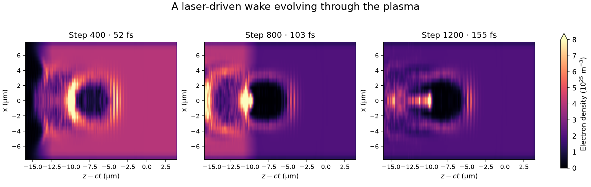
🫧 Find the cavity — electron density: a slice at y = 0 reveals the electron-depleted cavity and the surrounding concentration of electrons. The three-frame figure uses a shared color scale and the coordinate z−ct, which moves at the speed of light to keep the wake in view. Compare how the cavity changes as the laser crosses the density drop.
⚡ Find the push — longitudinal electric field, Ez: positive and negative regions show the direction of the field along the beam axis. Electrons have negative charge, so the longitudinal electric force is opposite to Ez. An electron moving forward can gain energy where this force points forward. In the single-snapshot figure, white contours on the density panel show the magnitude of Ey to help locate the pulse. Ey is the total transverse electric field and also includes plasma fields.
📈 Find the energetic electrons — the energy spectrum: the horizontal axis is kinetic energy and the vertical axis is charge magnitude per energy bin. Particle weights account for the physical electrons represented by each macroparticle. The spectrum includes all electrons in the moving window, not a selected bunch.

The single-snapshot density and field panels use laboratory z, while the three-frame density figure uses z−ct. Read the axis labels when comparing them. Choose a saved step during propagation: the last frame is after the moving window has passed the plasma and is less useful for viewing the wake.

💡 Follow the clues: locate the laser contours, then the cavity behind it. Find a region where the electric field would accelerate a forward-moving electron. Finally, inspect the energy spectrum. These views tell different parts of the same story; the spectrum alone does not show where those electrons are.

The notebook starts with a raw electron-charge histogram and a slice of the total transverse field Ey, which includes both laser and plasma fields. Its density-evolution plots use the moving coordinate z-ct. In the single-snapshot figure, white contours show |Ey|; the spectrum includes all electrons still in the moving box, including untrapped plasma electrons.

The fourth snapshot panel reads ParticleEnergy.txt and FieldEnergy.txt from diags/reducedfiles/, saved every simulation step. It compares total particle kinetic energy (all species) and electromagnetic field energy in mJ versus physical time in fs; the dashed line marks the selected snapshot. Laser injection and particles and fields crossing the moving box boundaries mean their sum need not stay constant. If these files are missing from an older run, preserve its diagnostics and rerun with the current input.

To save your figures without opening Jupyter, run these commands from laser-wakefield/:

BASH

python warpx_helpers.py diags/diag1 --evolution --output wake-evolution.png
python warpx_helpers.py diags/diag1 --iteration 800 --output wake-snapshot.png

Your turn: change one thing 🎛️

Keep the baseline input and results so you have something to compare with. Then choose one of these experiments. Make a prediction before rerunning!

Challenge

Turn the laser knob 🔦

Change my_constants.a0, the laser strength, and rerun. Compare the cavity, Ez, and spectrum at the same saved step. Does the cavity change shape? Does the high-energy part of the spectrum change too?

Alternatively, set n_up equal to n_down to remove the density drop while keeping the entrance and exit ramps. Watch how the wake evolves through the region where the drop used to be. Change one parameter at a time so you can connect a difference in the plots to a change in the input.

Challenge

Take fewer snapshots 📸

Change diag1.intervals from 200 to 400, then compare elapsed runtime, disk use (du -sh diags), and the available snapshots. What do you save in storage, and which moments can you no longer inspect?

The physical input and time steps are unchanged; only the saved history is less frequent. Compare a step saved in both runs. The computer still has to advance through every time step, even when it does not save a snapshot!

Challenge

Regular versus random particle placement

The raw electron histogram can show horizontal stripes: the baseline places one macroparticle per cell on a regular grid, and the histogram bins resolve those rows. Try randomizing the electron positions within each cell. In lwfa_warpx_input.txt, replace

electrons.injection_style = "NUniformPerCell"
electrons.num_particles_per_cell_each_dim = 1 1 1

with

electrons.injection_style = "NRandomPerCell"
electrons.num_particles_per_cell = 1

Remove the old num_particles_per_cell_each_dim line. Keep the density, grid, momentum distribution, and other settings fixed. These two loading styles use different particle-count parameters.

Preserve the baseline diagnostics before rerunning. Compare the electron histogram and deposited-density plot at the same saved step. Do the regular bands disappear? How much random variation appears instead?

This keeps one macroparticle per cell but changes its position. Random loading can replace regular sampling patterns with statistical noise and can affect the simulated fields, especially at this low particle count. A less striped plot alone does not demonstrate greater physical accuracy.

How far can we trust the picture? 🔍

A striking picture is a starting point for investigation. The compact laser and target make this visual demonstration practical. The simulation uses fixed, already-ionized helium ions, low particle sampling, and a grid that has not been refined to establish numerical convergence. It does not establish experimental beam quality or a target beam energy.

A wake and a high-energy tail demonstrate different things. Identifying a usable accelerated bunch also requires examining its spatial and momentum distribution, charge, and evolution after it leaves the plasma.

For other laser-wakefield configurations, including the role of geometry, see the official WarpX LWFA examples. The numerical choices here belong to this reduced teaching model and should be reassessed for a research calculation.

Key Points

🏄 A laser drives a plasma wake; its longitudinal field can accelerate electrons.
🧩 The grid, particles, and time steps determine which features are resolved and how much computation is required.
🔍 Density, field, and energy plots provide complementary evidence; an energy spectrum alone does not identify an accelerated bunch.
🎛️ Save the baseline and vary one setting at a time to interpret changes.